Handwriting Recognition using PyTorch

Overview

This project builds a deep learning model in PyTorch that reads human handwriting. A Convolutional Neural Network (CNN) is trained on the MNIST dataset to classify handwritten digits (0-9) straight from the raw image pixels - no hand-written rules, no manual feature extraction.

Instead of someone telling the program "a 7 has a horizontal bar and a diagonal stroke", the network learns those visual patterns by itself: first edges and strokes, then curves and corners, then whole-digit shapes. Training is monitored live in TensorBoard, and the final model reaches 93.46% accuracy on 10,000 unseen test images.

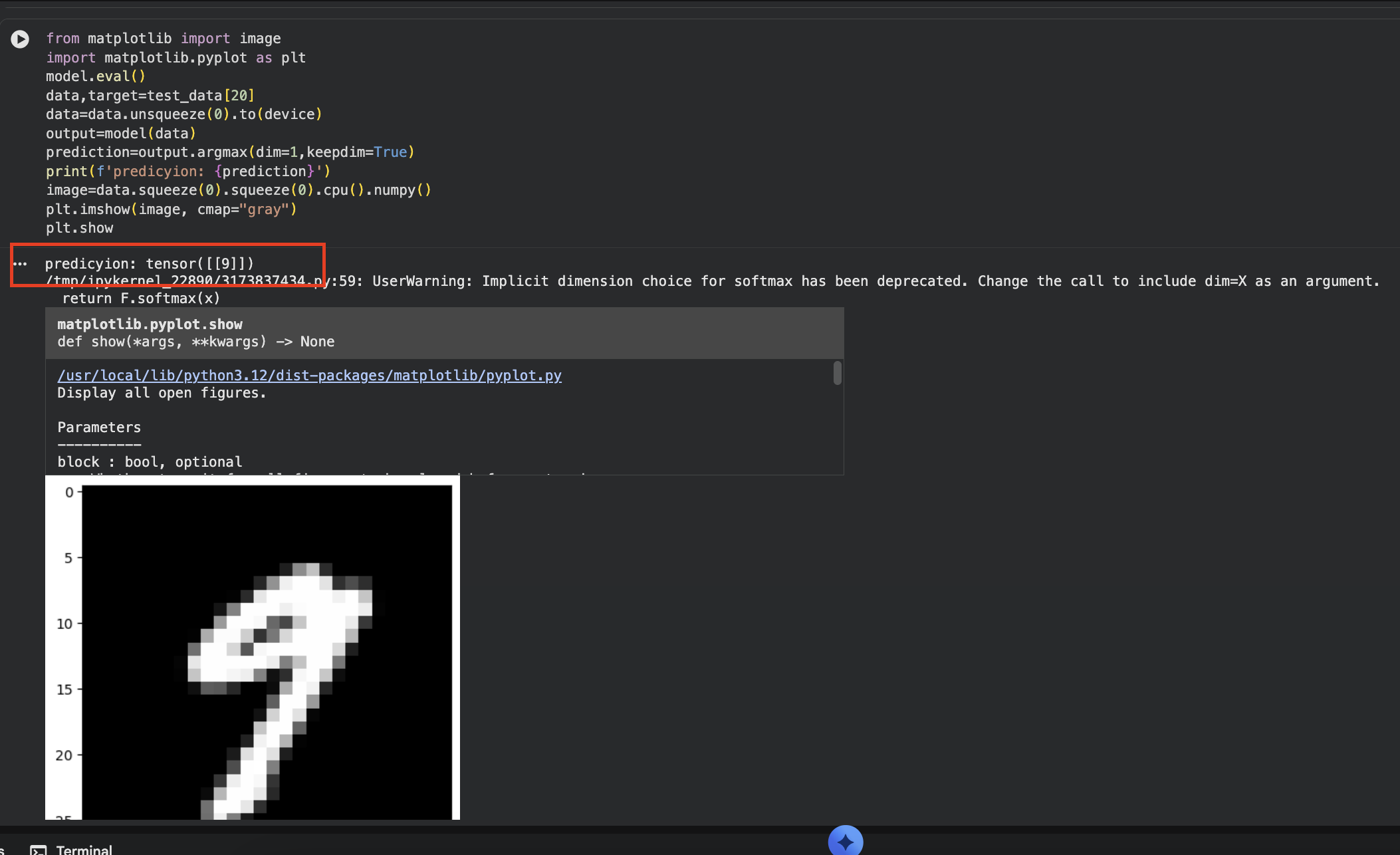
The trained model loading one image, switching to evaluation mode, and predicting a hand-drawn nine.

A few core concepts first

Before the code, here are the ideas this project is built on.

Deep learning

Deep learning is a branch of machine learning that stacks many layers of simple mathematical units ("neurons") on top of each other. Each layer transforms its input a little, and the depth (many layers) is what lets the network learn complex patterns. We never program the rules; we show the network thousands of examples and let it adjust its internal numbers (weights) until its guesses match the correct answers.

Neural network

A neural network is just a big function with many tunable numbers. You feed in an image and it outputs 10 scores - one per digit. Training is the process of nudging those numbers so the score for the correct digit becomes the highest.

Convolutional Neural Network (CNN)

A plain network treats every pixel independently and ignores the fact that nearby pixels form shapes. A CNN fixes this. It slides small filters (kernels, here 5×5) across the image. Each kernel acts like a tiny pattern detector - one might fire on vertical edges, another on curves. The result is a feature map that highlights where that pattern appears. Stack a few convolutional layers and the network builds features hierarchically:

• Layer 1: edges and strokes
• Layer 2: corners, loops, junctions
• Fully-connected layers: whole-digit shapes → the final decision

This is why CNNs are the standard tool for computer vision: they respect the 2D structure of an image and reuse the same kernel everywhere, so they need far fewer parameters than a fully-connected network.

"Class" - it means two things here

1. A class label is one of the categories we predict. This problem has 10 classes: the digits 0,1,2,…,9.
2. A Python class is how we define the model in PyTorch. We write class CNN(nn.Module) to package the layers and the forward pass into one reusable object.

Epoch, batch and iteration

• An epoch is one full pass over the entire training set (all 60,000 images). We train for 10 epochs, so the network sees the whole dataset ten times.
• A batch is a small group of images (here 100) processed together. We don't feed all 60,000 at once - too much memory, and small batches give smoother learning.
• One iteration = one batch. With 60,000 images and batch size 100 there are exactly 600 batches per epoch - which is why the logs below read Batch 0/600 … Batch 580/600.

Loss, optimizer and backpropagation

• The loss function measures how wrong the predictions are.
• Backpropagation computes how each weight contributed to that error.
• The optimizer (here Adam) uses those gradients to nudge every weight in the direction that reduces the loss. Repeat for every batch, every epoch, and the network slowly gets good.

Dataset - MNIST

The model is trained on MNIST: 70,000 grayscale images of handwritten digits - 60,000 for training, 10,000 for testing - each 28×28 pixels. It is the "hello world" of computer vision and the standard benchmark for this kind of task. We also create the TensorBoard SummaryWriter here so metrics can be logged from the very start.

from torchvision import datasets

from torchvision.transforms import ToTensor
from torch.utils.tensorboard import SummaryWriter

# Load the TensorBoard notebook extension
%load_ext tensorboard

writer = SummaryWriter("runs/cnn_experiment")



train_data=datasets.MNIST(
    root='data',
    train=True,
    transform=ToTensor(),
    download=True
    )
test_data=datasets.MNIST(
    root='data',
    train=False,
    transform=ToTensor(),
    download=True
    )

Quick sanity checks on the tensors - shapes, raw pixel values, and the labels:

train_data.data.shape

train_data.data[0]

train_data

test_data.data.shape

train_data.data

train_data.targets

Building the DataLoaders

A DataLoader serves the data in shuffled mini-batches of 100 during training, using a background worker so the GPU never waits for data.

from torch.utils.data import DataLoader


loaders={
    "train":DataLoader(train_data,
                        batch_size=100,
                        shuffle=True,
                        num_workers=1),
    "test":DataLoader(test_data,
                       batch_size=100,
                       shuffle=True,
                       num_workers=1)

}

loaders

Model architecture

A compact CNN: two convolutional layers (5×5 kernels) with 2D dropout and max pooling, then two fully-connected layers ending in a softmax over the 10 digit classes. This is the class that defines the model - the comments below walk through every layer and the dimension maths that gives the 320 flatten size.

The diagram below maps onto this network exactly: 28×28×1 input → Conv_1 (5×5) → 24×24 → Max-Pooling → 12×12 → Conv_2 (5×5) → 8×8 → Max-Pooling → 4×4, which flattens to 4×4×20 = 320, then fc_3 (320→50) and fc_4 (50→10).

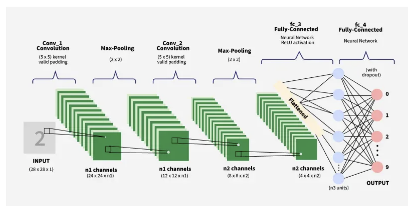
Image source: GeeksforGeeks - "Convolutional Neural Network (CNN) in Machine Learning" (geeksforgeeks.org). Used here for educational illustration; all rights remain with the original author.

import torch.nn as nn
## max pulling , softmax , relu and many more activation function
import torch.nn.functional as F

import torch.optim as optim

## creating the neural network architecture
## create a constructor to init the layers
## define convolution layers --> grayscale image ->1 and 1st conv to 10 filters output
## second layer conv2 input 10 and out the 20
## preventing model from learning all dropout some output from the conv2


class CNN(nn.Module):
  def __init__(self):
    super(CNN,self).__init__()

    self.conv1=nn.Conv2d(1,10,kernel_size=5)
    self.conv2=nn.Conv2d(10,20,kernel_size=5)
    self.conv2_drop=nn.Dropout2d()

   ## fully connected layer --> complex pattern connected to output
   ## formula: input-filter+1
   ## the size 320 --> 28 * 28 --> 5*5 filter --> 24*24 max pulling --> 12*12
   ## 12*12 --> (12-5)+1 --> 8 :::: 8*8 pixel ---> 4*4
   ## 4*4 --> 20  ---> 16*20 == 320 flatten
   ## 320 vector --> 50 neuron's input
   ## 10 output --> zero to nine == numbers

    self.fc1=nn.Linear(320,50)
    self.fc2=nn.Linear(50,10)

    ## now flow the data --> through convolution layer and nurons
    ## forward function --> network data flow --> layer to layer
    ## x is tensor
    ## relu ---> rectified linear unit ---> make them non liniearity
       ## negative --> 0 positive as it is
    ## max pool for saving memory and computation
    ## conv1 maxpool half --> relu add --> non linear
    ## conv2_drop --> the same

  def forward(self,x):
    x=F.relu(F.max_pool2d(self.conv1(x),2))
    x=F.relu(F.max_pool2d(self.conv2_drop(self.conv2(x)),2))

      ## conv2 --> output should be flatten before sending to neurons
      ## batch size calculation
      ## flatten (-1 for calcuting batch size when different size is encounter)

    x= x.view(-1,320)

      #first dense layer
    x=F.relu(self.fc1(x))
      ## remove overfitting
    x=F.dropout(x,training=self.training)
    x=self.fc2(x)

      ## softnax --> convert to probability
    return F.softmax(x)

Training the model

The model is moved to the GPU (if available), optimised with Adam (lr=0.0001) and cross-entropy loss. The train function loops over the ~600 batches in an epoch, runs the forward/backward pass, updates the weights, and logs the training loss to TensorBoard each step.

import torch

from torch.nn.modules import loss
device=torch.device("cuda" if torch.cuda.is_available() else "cpu")
model=CNN().to(device)

## adam --> adaptive movement estimation
## pytorch optimizer algorithm
## gradient decent + moment RMS

optimizer=optim.Adam(model.parameters(),lr=0.0001)

loss_fn= nn.CrossEntropyLoss()

def train(epoch):
  model.train()

  ## dataset is too large so creating the batches in loop to train the model
  ## enumerate:
  ## fruits = ["apple", "banana", "cherry"]
  ## for index, fruit in enumerate(fruits):
  ## print(f"Index {index}: {fruit}")

  for batch_idx,(data,target) in enumerate(loaders["train"]):

    ## sending data and target to gpu
    data, target = data.to(device),target.to(device)

    ## zero_grad = reset all the gradient ; preventing grad addition in next loop
    optimizer.zero_grad()

    ## storing the output ---> passing the data (input) to the model
    output=model(data)

    loss=loss_fn(output,target)

    ## back propagation --> network parameter --> store gradient tensor
    loss.backward()

    ## gradient -->> change the weights
    optimizer.step()

    ## global step for tensorboard
    step = epoch * len(loaders["train"]) + batch_idx

    ## using the tensorboard for visulization
    writer.add_scalar("Loss/Train", loss.item(), step)

    if batch_idx % 20 == 0:
      print(
          f"Epoch {epoch} | "
          f"Batch {batch_idx}/{len(loaders['train'])} | "
          f"Loss: {loss.item():.4f}"
      )

Evaluation

The test function switches the model to evaluation mode, runs over the held-out test set inside torch.no_grad() (no gradients needed), accumulates the loss, counts correct predictions with argmax, and logs both loss and accuracy to TensorBoard.

## now for testing
def test(epoch):

  ## convert the model to evaluation mode
  model.eval()

  ## zero fresh --> remove garbage
  test_loss=0
  correct=0

  ## no need to remember the gradient
  ## for --> to all data
  with torch.no_grad():

    for data,target in loaders["test"]:

      data,target=data.to(device),target.to(device)

      output=model(data)

      ## criterian
      ## batch loss sum up
      test_loss += loss_fn(output,target).item()

      ## dim --> 0 means batch and dim = 1 --> model pred score
      ## keepdim = true output and input same dimension
      pred=output.argmax(dim=1, keepdim=True)

      ## target.view_as --> reshape target and prediction same
      ## pred.eq ---> compares elementwise : true and false
      ## sum up all batches
      correct += pred.eq(target.view_as(pred)).sum().item()

  ## average loss over batches
  test_loss /= len(loaders["test"])

  test_accuracy = 100. * correct / len(loaders["test"].dataset)

  ## tensorboard logging
  writer.add_scalar("Loss/Test", test_loss, epoch)
  writer.add_scalar("Accuracy/Test", test_accuracy, epoch)

  print(
      f"\nTest Set: "
      f"Average Loss: {test_loss:.4f}, "
      f"Accuracy: {correct}/{len(loaders['test'].dataset)} "
      f"({test_accuracy:.2f}%)\n"
  )

Running the loop & launching TensorBoard

Train and evaluate for 10 epochs, then open the TensorBoard dashboard inline.

for epoch in range (1,11):
  train(epoch)
  test(epoch)

%tensorboard --logdir runs

TensorBoard is a dashboard for watching training in real time. Throughout the run, writer.add_scalar(...) streams Loss/Train, Loss/Test and Accuracy/Test to the runs/ folder, and %tensorboard --logdir runs renders them. The accuracy curve climbs steeply in the first epochs and then flattens as the model converges - the classic learning curve shape.

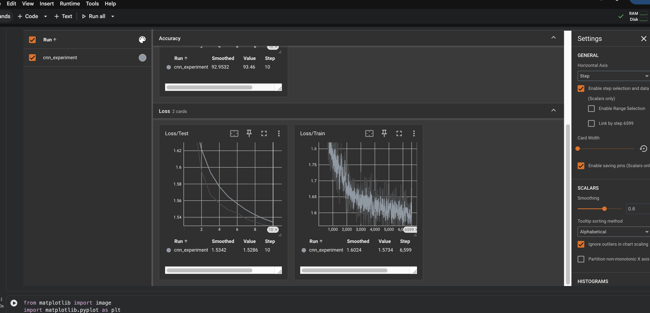
TensorBoard dashboard. The cnn_experiment run reporting Accuracy 93.46, Loss/Test 1.5286 and Loss/Train 1.5734 at the final step.

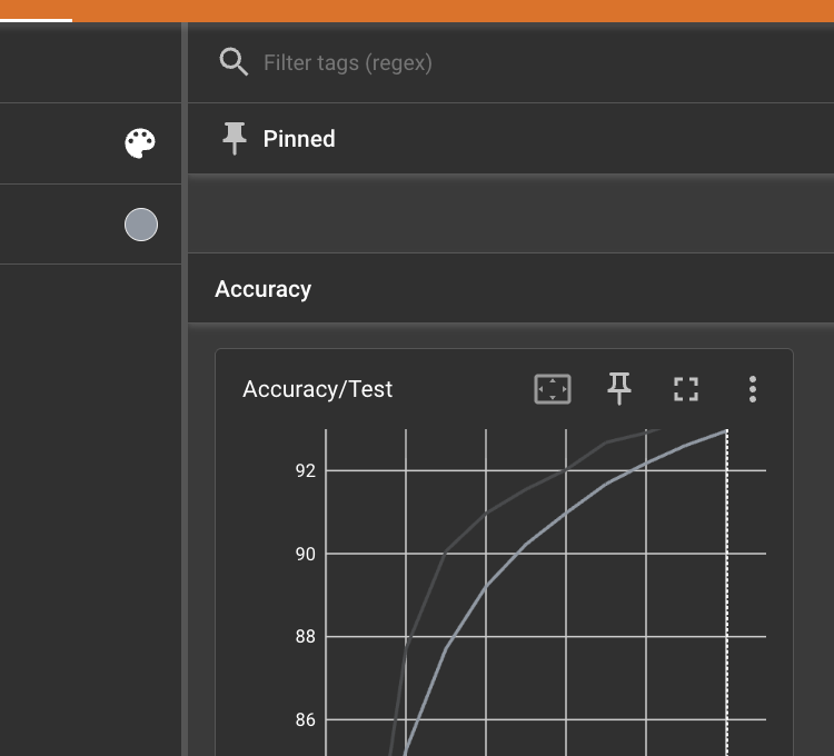
Accuracy/Test curve. Test accuracy rises from ~86% to ~93% over the run, with the gains flattening out as training converges.

Results

Final-epoch (epoch 10) training log, printed every 20 batches across the 600 batches in the epoch:

Epoch 10 | Batch 0/600   | Loss: 1.6238
Epoch 10 | Batch 20/600  | Loss: 1.6134
Epoch 10 | Batch 40/600  | Loss: 1.6074
Epoch 10 | Batch 60/600  | Loss: 1.5904
Epoch 10 | Batch 80/600  | Loss: 1.5615
Epoch 10 | Batch 100/600 | Loss: 1.5901
Epoch 10 | Batch 120/600 | Loss: 1.6192
Epoch 10 | Batch 140/600 | Loss: 1.5908
Epoch 10 | Batch 160/600 | Loss: 1.6080
Epoch 10 | Batch 180/600 | Loss: 1.6009
Epoch 10 | Batch 200/600 | Loss: 1.5980
Epoch 10 | Batch 220/600 | Loss: 1.5928
Epoch 10 | Batch 240/600 | Loss: 1.5754
Epoch 10 | Batch 260/600 | Loss: 1.5804
Epoch 10 | Batch 280/600 | Loss: 1.6197
Epoch 10 | Batch 300/600 | Loss: 1.5844
Epoch 10 | Batch 320/600 | Loss: 1.5961
Epoch 10 | Batch 340/600 | Loss: 1.6315
Epoch 10 | Batch 360/600 | Loss: 1.5607
Epoch 10 | Batch 380/600 | Loss: 1.5871
Epoch 10 | Batch 400/600 | Loss: 1.6470
Epoch 10 | Batch 420/600 | Loss: 1.5551
Epoch 10 | Batch 440/600 | Loss: 1.6743
Epoch 10 | Batch 460/600 | Loss: 1.5794
Epoch 10 | Batch 480/600 | Loss: 1.6022
Epoch 10 | Batch 500/600 | Loss: 1.5681
Epoch 10 | Batch 520/600 | Loss: 1.6219
Epoch 10 | Batch 540/600 | Loss: 1.5677
Epoch 10 | Batch 560/600 | Loss: 1.5976
Epoch 10 | Batch 580/600 | Loss: 1.5435

Final evaluation on the 10,000-image test set:

Test Set: Average Loss: 1.5309, Accuracy: 9325/10000 (93.25%)
Test Set: Average Loss: 1.5286, Accuracy: 9346/10000 (93.46%)

The model correctly classifies 9,346 out of 10,000 unseen digits - 93.46% accuracy. (The loss sits near 1.5 rather than near 0 because the forward pass already applies F.softmax and nn.CrossEntropyLoss applies log-softmax internally as well, so accuracy is the reliable signal to read here.)

Inference on a single image

Finally, load one test image, run it through the trained model, print the predicted digit, and display the image with Matplotlib.

from matplotlib import image
import matplotlib.pyplot as plt
model.eval()
data,target=test_data[20]
data=data.unsqueeze(0).to(device)
output=model(data)
prediction=output.argmax(dim=1,keepdim=True)
print(f'predicyion: {prediction}')
image=data.squeeze(0).squeeze(0).cpu().numpy()
plt.imshow(image, cmap="gray")
plt.show

This is the snippet behind the screenshot at the top of the page - the model reads the drawn digit and prints its prediction.

Key insight

A CNN can learn to read human handwriting straight from raw pixels, with no manual feature engineering. The same architecture extends naturally to letters and full handwritten words. The biggest practical lesson is that a model which scores 93% on MNIST can still fail on your own drawings, because your input has to be preprocessed to look like MNIST (centred, 28×28, white-on-black, normalised) before the model has a fair chance.

Tech stack

• PyTorch & TorchVision - model, training loop, dataset utilities
• Convolutional Neural Network (CNN) - two conv blocks + fully-connected head
• MNIST dataset - 70,000 handwritten-digit images
• Adam optimizer & cross-entropy loss
• TensorBoard (torch.utils.tensorboard.SummaryWriter) - live metric tracking
• Matplotlib - visualising input images and predictions

Reference

• MNIST - The MNIST Database of Handwritten Digits
• TensorBoard - TensorFlow's Visualization Toolkit
• GeeksforGeeks - Convolutional Neural Network (CNN) in Machine Learning (CNN diagram source)
• NeuralNine. (2026, June 17). PyTorch Project: Handwritten Digit Recognition.